This document describes my experience in developing a C++ implementation of some onset detection algorithms. The departure point is taken as that described by Klapuri in [Kla99]. His approach is informed by the current level of understanding of the Human Auditory System (HAS), particularly as described by B. J. Moore. Klapuri's paper is available here, and he announed it here.
The algorithm has three principal stages. First, digital audio data is normalised to have a sound level of 70dB, according to the model described by Mooore. Then, the normalised signal is split into bands, and for each band the decimated envelope is found, convolved with a half-Hann window, and has onset detection applied. Finally, the results from each envelope are combined.
I haven't implemented this yet (because the library can't find the relevant journal)
The first requirement here is to set up a filterbank of gammatone filters, for which I'm using the Matlab Auditory Toolbox by Malcolm Slaney (available here). I wrote a Matlab script which uses the functions from the Toolbox to generate .cpp and .h files with filter coefficients for specified sample rates and frequency range. These coefficients are used to initialise several 'cascade of biquad' filters, for which I use the Intel IPP library. My implementation uses doubles for filter coefficients, but samples are stored as 32-bit float. At present, I use a 32-band bank with filters ranging from 44Hz to 9.79kHz (spaced using ERBSpace from the Auditory Toolbox).
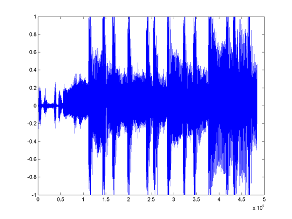
Each band is then decimated, full-rectified, and convolved with a half-Hann window of length 100ms (temporal integration). These stages are illustrated below for a short clip from a techno mix by Laurent Garnier, sampled at 44.1kHz (click to hear it):
As regards onset detection, we might reasonably hope to get the bass, ride cymbal and snare from this, and perhaps the synth changes. The synth changes are, in approximate sample offsets, at 55500, 92091, 145160, 243790, 284886, 375590, 408590, 441730, and 464260 (determined by laborious listening and a bit of spectrogramming).
Here are the lowest, middle, and highest filter outputs (central frequencies 44, 1523, and 9790 Hz) (click to hear them). On the right are the integrated, decimated envelopes (decimation factor is 180, so envelope resolution ~= 4ms).
 |
 |
The bass has been picked out by this filter quite well; the peaks in the integrated envelope correspond to the bass sounds. |
|
 |
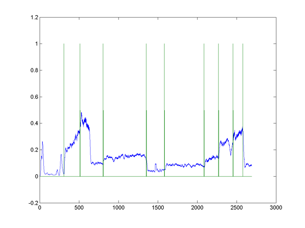 |
This band is mostly synth; the approximate synth changepoints are at the green lines. It's apparent that sudden changes in the filter output are correlated with the synth tone, but sometimes these changes are small. |
|
 |
 |
Here we have the cymbal and the snare, distinguished by their amplitude. | |
At this juncture, it's evident that for the drum sounds, we could easily get away with peak picking / thresholding in the envelopes. However, the synth changes are not at all so obvious. Since we can reasonably argue that drum sounds are usually more important in determining the rhythm, we might as well start by developing a method to detect them.
It seems in the graphs that the peaks generally rise faster than they fall -- this is (mostly) a consequence of the half-Hanning window. So we'll focus on detecting a sharp rise in the envelopes. What might work, is detecting where the envelope rises above the mean of the last 'few' values. Illustrated with Matlab code:
 band=32; thresh=2;
 ampWin = 32; diff2 = differenced(:,band); diff2(1:ampWin,band)=0;
 for i=ampWin:length(integrated(:,band))
  if (integrated(i,band) < thresh*mean(integrated(i-(ampWin-1):i,band))) diff2(i)=0; end;
 end
 plot([integrated(:,band) diff2]);shg
In this code, band is which band to analyse, and
thresh is the factor by which the peak must exceed
the mean. ampWin is the size of the window to
consider (it's a causal window). differenced is the
relative difference of integrated, which in turn is
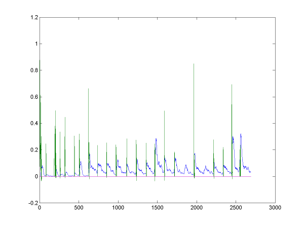
the downsampled, temporally integrated envelope. The graphs below,
show the peaks , with the detection track in green (bass on the
left, high band on the right).
Winsize = 16 (64ms) (thresh = 2) |
|
 |
 |
Winsize = 32 (128ms) (thresh = 2) |
|
 |
 |
Winsize = 64 (256ms) (thresh = 2) |
|
 |
 |
We see that the 64-tap window is the most successful at detecting the peaks in both envelopes. Only the 16-sample window found the cymbal peak at offset ~750, but then it missed the peaks at either side of 2000. A disadvantage of using the 64-sample window is that it the signal is being averaged over more than a quarter of a second, which means that drum onsets that succeed each other in less than this time (which could easily happen) might be missed.
What might improve matters? The peaks are definitely there, but they sometimes rise more slowly than at other times. We could try to mitigate the effect of this by computing the mean of a window a few samples back from the point under consideration -- here's some more Matlab for those that way inclined:
band=1; thresh=1.5; winDelay=6;
ampWin = 16; diff2 = differenced(:,band); diff2(1:(ampWin+winDelay),band)=0;
for i=(ampWin + winDelay):length(integrated(:,band))
 if (integrated(i,band) < thresh*mean(integrated((i-ampWin-winDelay+1):(i-winDelay),band))) diff2(i)=0; end;
end
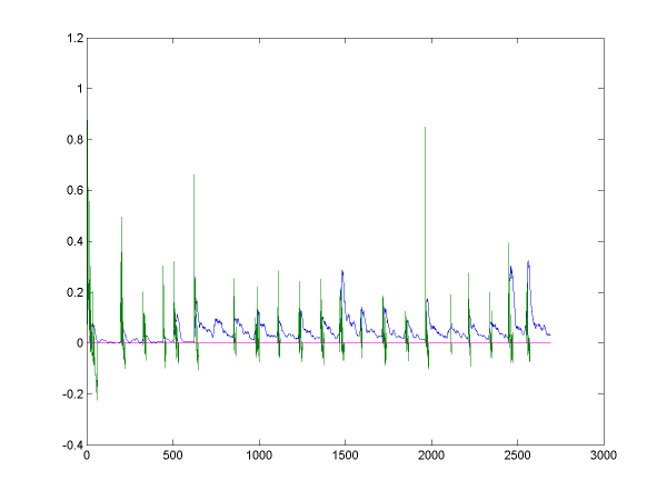
And this works pretty good; in particular, the result for the bass
band is much better. Results for the two bands are shown below
(note that the thresh has been decreased to 1.5 here). We have a
temporal granularity of about (16+6)*4 = 80ms, which is a sizeable
improvement. Some false alarms have crept in here, but for this
application I think recall is more important than precision.
 |
 |